
Error Data in Weather Radar
In the sky there is more than rain and snow. Other objects can be misinterpreted as rain by a weather radar. The main ones are[10]:
* Birds, especially in period of migration.
* Insects at low altitude.
* Thin metal strips (chaff) dropped by military aircraft to fool enemies.
* Solid obstacles such as mountains, buildings, and aircraft.
* Ground and sea clutter.
* Reflections from buildings if the radar is close enough to a city (called urban spikes).
Each of them has their own characteristics that make it possible to distinguish them to the trained eye but they may fool a layman. It is possible to eliminate some of them with post-treatment of data using reflectivity, Doppler, and polarization data.
Type Data Output from weather Radar : others
Accumulations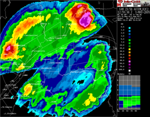 One of the main use of radar is to be able to assess the amount of precipitations fallen over large basins for hydrological purpose. For instance, river flood control, sewer management and dam construction are all areas where planners want accumulation data. It ideally completes surface stations data which they can use for calibration.
To produce radar accumulations, we have to estimate the rain rate over a point by the average value over that point between one PPI, or CAPPI, and the next; then multiply by the time between those images. If one wants for a longer period of time, one has to add up all the accumulations from images during that time.
Echotops
Aviation is a heavy user of radar data. One map particularly important in this field is the Echotops for flight planning and avoidance of dangerous weather. Most country weather radars are scanning enough angles to have a 3D set of data over the area of coverage. It is relatively easy to estimate the maximum altitude at which precipitation is found within the volume. However, those are not the tops of clouds as they extended to higher altitudes than the precipitation.
Vertical cross sections
To know the vertical structure of clouds, in particular thunderstorms or the level of the melting layer, a vertical cross sections product of the radar data is available to meteorologist. This is done by displaying only the data along a line, from coordinates A to B, taken from the different angles scanned.
Range Height Indicator
When a weather radar is scanning in only one direction vertically, it obtains high resolution data along a vertical cut of the atmosphere. The output of this sounding is called a Range Height Indicator (RHI) which is excellent for viewing the detailed vertical structure of a storm. This is different from the vertical cross section mentioned above by the fact that the radar is making a vertical cut along specific directions and does not scan over the entire 360 degrees around the site. This kind of sounding and product is only available on research radars.
Radar networks
Over the past few decades, radar networks have been extended to allow the production of composite views covering large areas. For instance, all major countries (e.g., the United States, Canada, much of Europe) produce images that include all of their radars. This is not as trivial a task.
In fact, such a network can consist of different types of radar with different characteristics like beam width, wavelength and calibration. These differences have to be taken into account when matching data across the network, particularly to decide what data to use when two radars cover the same point. If one uses the stronger echo but it comes from the most distant radar, one uses returns that are from higher altitude coming from rain or snow that might evaporate before reaching the ground (virga). If one uses data from the closest radar, it might be attenuated passing through a thunderstorm. Composite images of precipitations using a network of radars are made with all those limitations in mind.
Type Data Output from Weather Radar : Animation
 The animation of radar products can show the evolution of reflectivity and velocity patterns. The user can extract information on the dynamics of the meteorological phenomena, including the ability to extrapolate the motion and observe development or dissipation. This can also reveal non-meteorological artifacts (false echoes) that will be discussed later.
Type Data Output from Weather Radar : VIL
VERTICAL INTEGRATED LIQUID Automatic algorithmsTo help meteorologists to spot dangerous weather, mathematical algorithms have been introduced in the weather radar treatment programs. These are particularly important in the analyzing the Doppler velocity data as they are more complex. The polarization data will even need more algorithms.
Main algorithms for reflectivity[7]:
* Vertically Integrated Liquid (VIL) is an estimate of the total mass of precipitation in the clouds.
* Potential wind gust, which can estimate the winds under a cloud (a downdraft) using the VIL and the height of the echotops (radar estimated top of the cloud) for a given storm cell.
* Hail algorithm that estimates the presence and potential size.
Main algorithms for Doppler velocities[7]:
* Mesocyclone detection: it is triggered by a velocity change over a small circular area. The algorithm is searching for a "doublet" of inbound/outbound velocities with the zero line of velocities, between the two, along a radial line from the radar. Usually the mesocyclone detection must be found on two or more stacked progressive tilts of the beam to be significative of rotation into a thunderstom cloud.
* TVS or Tornado Vortex Signature algorithm is essentially a mesocyclone with a large velocity threshold found through many scanning angles. This algorithm is used in NEXRAD to indicate the possibility of a tornado formation.
* Wind shear in low levels. This algorithm detects variation of wind velocities from point to point in the data and looking for a doublet of inbound/outbound velocities with the zero line perpendicular to the radar beam. The wind shear is associated with downdraft, (downburst and microburst), gust fronts and turbulence under thunderstorms.
* VAD Wind Profile (VWP) is a display that estimates the direction and speed of the horizontal wind at various upper levels of the atmosphere, using the technique explained in the Doppler section.
Type Data Output fro Weather Radar : VC
Vertical composite
Another solution to the PPI problems is to produce images of the maximum reflectivity in a layer above ground. This solution is usually taken when the number of angles available is small or variable. The American National Weather Service is using such Composite as their scanning scheme can vary from 4 to 14 angles, according to their need, which would make very coarse CAPPIs. The Composite make sure that no strong echo is missed in the layer and a treatment using Doppler velocities eliminate the ground echoes. Comparing base and composite products, one can locate virga and updrafts zones.Type Data Output from Weather Radar : CAPPI
Constant Altitude Plan Position Indicator
To avoid some of the problems on PPIs, the CAPPI or Constant Altitude Plan Position Indicator has been developed by researchers in Canada. It is basically a horizontal cross-section through radar data. This way, one can compare precipitation on an equal footing at difference distance from the radar and avoid ground echoes. Although data are taken at a certain height above ground, a relation can be inferred between ground stations reports and the radar data.CAPPIs call for a large number of angles from near the horizontal to near the vertical of the radar in order to have a cut that is as close as possible at all distance to the height needed. But even then, after a certain distance, there isn’t any angle available and the CAPPI becomes the PPI of the lowest angle. The zigzag line on the angles diagram above shows the data used to produce a 1.5 and 4 km height CAPPIs. Notice that the section after 120 km is using the same data.
USAGE: Mostly for reflectivity data. McGill University is producing Doppler CAPPIs but the nature of velocity make the output a bit noisy as velocities can change rapidly in direction with height contrary to a relatively smooth pattern in reflectivity.
Type Data Output from Weather Radar : PPI
Plan position indicator
 Since data are obtained one angle at a time, the first way of displaying them as been the Plan Position Indicator (PPI) which is only the layout of radar return on a two dimensional image. One has to remember that the data coming from different distances to the radar are at different heights above ground.
This is very important as a high rain rate seen near the radar is relatively close to what reach the ground but what is seen from 160 km (100 miles) away is about 1.5 km above ground and could be far different from the amount reaching the surface. It is thus difficult to compare weather echoes at different distance from the radar.
PPIs are afflicted with ground echoes near the radar as a supplemental problem. These can be misinterpreted as real echoes. So other products and further treatments of data have been developed to supplement its shortcomings.
USAGE: Reflectivity, Doppler and polarimetric data can use PPI.
N.B.: In the case of Doppler data, two points of view are possible: relative to the surface or the storm. When looking at the general motion of the rain to extract wind at different altitudes, it is better to use data relative to the radar. But when looking for rotation or wind shear under a thunderstorm, it is better to use the storm relative images that subtract the general motion of precipitation leaving the user to view the air motion as if he would be sitting on the cloud.
How Weather Radar Work (Part.4)
Calibrating intensity of return
Because the targets are not unique in each volume, the radar equation has to be developed beyond the basic one[7]: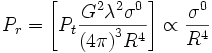 where \,P_r is received power, \,P_t is transmitted power, \,G_t is the gain of the transmitting antenna, \,\lambda is radar wavelength, \,\sigma is the radar cross section of the target and \,R is the distance from transmitter to target.
In this case, we have to add the cross sections of all the targets:

 where \,c is the light speed, \,\tau is temporal duration of a pulse and \,\theta is the beam width in radians.
In combining the two equations :

Which leads to:
 Notice that the return now varies inversely to \, R^2 instead of \,R^4. In order to compare the data coming from different distances from the radar, one has to normalize them with this ratio.
How Weather Radar Work (Part.3)
Determining height
 Assuming the Earth is round, with knowledge of the variation of the index of refraction through air and the distance to the target, one can calculate the height above ground of the target.
After each scanning rotation, the antenna elevation is changed for the next sounding. This scenario will be repeated on many angles in order to scan all the volume of air around the radar within the maximum range. Usually, this scanning strategy is completed within 5 to 10 minutes in order to have data within 15 km above ground and 250 km distance of the radar.

Due to the Earth curvature and change of index of refraction with height, the radar cannot “see” below the height above ground of the minimal angle or closer to the radar than the maximal one. This image shows the height of a series of typical angles done by a 5 cm weather radar in Canada. They range from 0.3 to 25 degrees.
How Weather Radar Work (Part.2)
Listening for return signals
Between each pulse, the radar station serves as a receiver and listens for return signals from particles in the air. The duration of the "listen" cycle is on the order of a millisecond, which is a thousand times longer than the pulse duration. The length of this phase is determined by the need for the microwave radiation (which travels at the speed of light) to propagate from the detector, to the weather target, and back again, a distance which could be several hundred kilometers. The horizontal distance from station to target is calculated simply from the amount of time that lapses from the initiation of the pulse to the detection of the return signal. (The time is converted into distance by multiplying by the speed of light). If pulses are emitted too frequently, the returns from one pulse will be confused with the returns from previous pulses, resulting in incorrect distance calculations.How Weather Radar Work (Part.1)
Sending radar pulses
 Weather radars send directional pulses of microwave radiation, on the order of a microsecond long, using a cavity magnetron or klystron tube connected by a waveguide to a parabolic antenna. The wavelengths of 1 to 10 cm are approximately ten times the diameter of the droplets or ice particles of interest, because Rayleigh scattering occurs at these frequencies. This means that part of the energy of each pulse will bounce off these small particles, back in the direction of the radar station[7].
Shorter wavelengths are useful for smaller particles, but the signal is more quickly attenuated. Thus 10 cm (S-band) radar is preferred to but is more expensive than a 5 cm C-band system. 3 cm X-band radar is used only for very short distance purposes, and 1 cm Ka-band weather radar is used only for research on small-particle phenomena such as drizzle and fog[7].
Radar pulses spread out as they move away from the radar station. This means that the region of air any given pulse is moving through is larger for areas farther away from the station, and smaller for nearby areas, decreasing resolution at far distances. At the end of a 150-200 km sounding range, the volume of air scanned by a single pulse might be on the order of a cubic kilometer.
The volume of air that a given pulse takes up at any point in time may be approximately calculated by the formula \, {v = h r^2 \theta^2}, where v is the volume enclosed by the pulse, h is pulse width (in e.g. meters, calculated from the duration in seconds of the pulse times the speed of light), r is the distance from the radar that the pulse has already traveled (in e.g. meters), and \,\theta is the beam width in radians). This formula assume the beam is symmetrically circular, "r" is much greater than "h" so "r" taken at the beginning or at the end of the pulse is almost the same, and the shape of the volume is a cone frustum of depth "h"[7].
History of Weather Radar
 During World War II, military radar operators noticed noise in returned echoes due to weather elements like rain, snow, and sleet. Just after the war, military scientists returned to civilian life or continued in the Armed Forces and pursued their work in developing a use for those echoes. In the United States, David Atlas,[1] for the Air Force group at first, and later for MIT, developed the first operational weather radars. In Canada, J.S. Marshall and R.H. Douglas formed the "Stormy Weather Group[2]" in Montreal. Marshall and his doctoral student Walter Palmer are well known for their work on the drop size distribution in mid-latitude rain that led to understanding of the Z-R relation, which correlates a given radar reflectivity with the rate at which water is falling on the ground. In the United Kingdom, research continued to study the radar echo patterns and weather elements such as stratiform rain and convective clouds, and experiments were done to evaluate the potential of different wavelengths from 1 to 10 centimetres.
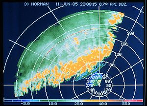
In 1953, Donald Staggs, an electrical engineer working for the Illinois State Water Survey, made the first recorded radar observation of a "hook echo" associated with a tornadic thunderstorm. [3]
Between 1950 and 1980, reflectivity radars, which measure position and intensity of precipitation, were built by weather services around the world. The early meteorologists had to watch a cathode ray tube. During the 1970s, radars began to be standardized and organized into networks. The first devices to capture radar images were developed. The number of scanned angles was increased to get a three-dimensional view of the precipitation, so that horizontal cross-sections (CAPPI) and vertical ones could be performed. Studies of the organization of thunderstorms were then possible with the Alberta Hail Project in Canada and NSSL in the US in particular. NSSL, created in 1964, began experimentation on dual polarization signals and on Doppler effect uses.
Between 1980 and 2000, weather radar networks became the norm in North America, Europe, Japan and other developed countries. Conventional radars were replaced by Doppler radars, which in addition to position and intensity of could track the relative velocity of the particles in the air. In the United States, a network consisting of 10 cm wavelength radars, called NEXRAD or WSR-88D (Weather Service Radar 1988 Doppler), was started in 1988. In Canada, Environment Canada constructed the King City station,[4] with a five centimeter research Doppler radar, by 1985;McGill University dopplerized its radar (J. S. Marshall Radar Observatory) in 1993. This led to a complete Canadian Doppler network[5] between 1998 and 2004. France and other European countries switched to Doppler network by the end of the 1990s to early 2000s. Meanwhile, rapid advances in computer technology led to algorithms to detect signs of severe weather and a plethora of "products" for media outlets and researchers.
After 2000, research on dual polarization technology has moved into operational use, increasing the amount of information available on precipitation type (e.g. rain vs. snow). "Dual polarization" means that microwave radiation which is polarized both horizontally and vertically (with respect to the ground) is emitted. Wide-scale deployment is expected by the end of the decade in some countries such as the United States, France,[6] and Canada.
Since 2003, the U.S. National Oceanic and Atmospheric Administration has been experimenting with phased-array radar as a replacement for conventional parabolic antenna in order to provide more time resolution in atmospheric sounding. This would be very important in severe thunderstorms as their evolution can be better evaluated with more timely data.
Tools : Weather Radar
A weather radar is a type of radar used to locate precipitation, calculate its motion, estimate its type (rain, snow, hail, etc.), and forecast its future position and intensity. Modern weather radars are mostly pulse-doppler radars, capable of detecting the motion of rain droplets in addition to intensity of the precipitation. Both types of data can be analyzed to determine the structure of storms and their potential to cause severe weather.
Subclassion of Meteorology
In the study of the atmosphere, meteorology can be divided into distinct areas of emphasis depending on the temporal scope and spatial scope of interest. At one extreme of this scale is climatology. In the timescales of hours to days, meteorology separates into micro-, meso-, and synoptic scale meteorology. Respectively, the geospatial size of each of these three scales relates directly with the appropriate timescale.
Other subclassifications are available based on the need by or by the unique, local or broad effects that are studied within that sub-class.
Boundary layer meteorologyBoundary layer meteorology is the study of processes in the air layer directly above Earth's surface, known as the atmospheric boundary layer (ABL) or peplosphere. The effects of the surface – heating, cooling, and friction – cause turbulent mixing within the air layer. Significant fluxes of heat, matter, or momentum on time scales of less than a day are advected by turbulent motions. Boundary layer meteorology includes the study of all types of surface-atmosphere boundary, including ocean, lake, urban land and non-urban land.
Mesoscale meteorologyMesoscale meteorology is the study of atmospheric phenomena that has horizontal scales ranging from microscale limits to synoptic scale limits and a vertical scale that starts at the Earth's surface and includes the atmospheric boundary layer, troposphere, tropopause, and the lower section of the stratosphere. Mesoscale timescales last from less than a day to the lifetime of the event, which in some cases can be weeks. The events typically of interest are thunderstorms, squall lines, fronts, precipitation bands in tropical and extratropical cyclones, and topographically generated weather systems such as mountain waves and sea and land breezes.
Synoptic scaleSynoptic scale meteorology is generally large area dynamics referred to in horizontal coordinates and with respect to time. The phenomena typically described by synoptic meteorology include events like extratropical cyclones, baroclinic troughs and ridges, frontal zones, and to some extent jets. All of these are typically given on weather maps for a specific time. The minimum horizontal scale of synoptic phenomena are limited to the spacing between surface observation stations.
Global scaleGlobal scale meteorology is study of weather patterns related to the transport of heat from the tropics to the poles. Also, very large scale oscillations are of importance. Those oscillations have time periods typically longer than a full annual seasonal cycle, such as ENSO, PDO, MJO, etc. Global scale pushes the thresholds of the perception of meteorology into climatology. The traditional definition of climate is pushed in to larger timescales with the further understanding of how the global oscillations cause both climate and weather disturbances in the synoptic and mesoscale timescales.
Numerical Weather Prediction is a main focus in understanding air-sea interaction, tropical meteorology, atmospheric predictability, and tropospheric/stratospheric processes.Currently (2007) Naval Research Laboratory in Monterey produces the atmospheric model called NOGAPS, a global scale atmospheric model, this model is run operationally at Fleet Numerical Meteorology and Oceanography Center. There are several other global atmospheric models.
Dynamic meteorologyDynamic meteorology generally focuses on the physics of the atmosphere. The idea of air parcel is used to define the smallest element of the atmosphere, while ignoring the discrete molecular and chemical nature of the atmosphere. An air parcel is defined as a point in the fluid continuum of the atmosphere. The fundamental laws of fluid dynamics, thermodynamics, and motion are used to study the atmosphere. The physical quantities that characterize the state of the atmosphere are temperature, density, pressure, etc. These variables have unique values in the continuum.
Aviation meteorologyAviation meteorology deals with the impact of weather on air traffic management. It is important for air crews to understand the implications of weather on their flight plan as well as their aircraft, as noted by the Aeronautical Information Manual:
The effects of ice on aircraft are cumulative-thrust is reduced, drag increases, lift lessens, and weight increases. The results are a decrease in stall speed and a deterioration of aircraft performance. In extreme cases, 2 to 3 inches of ice can form on the leading edge of the airfoil in less than 5 minutes. It takes but 1/2 inch of ice to reduce the lifting power of some aircraft by 50 percent and increases the frictional drag by an equal percentage.
Meteorologists, soil scientists, agricultural hydrologists, and agronomists are persons concerned with studying the effects of weather and climate on plant distribution, crop yield, water-use efficiency, phenology of plant and animal development, and the energy balance of managed and natural ecosystems. Conversely, they are interested in the role of vegetation on climate and weather.
Agricultural meteorology
HydrometeorologyHydrometeorology is the branch of meteorology that deals with the hydrologic cycle, the water budget, and the rainfall statistics of storms.[11] A hydrometeorologist prepares and issues forecasts of accumulating (quantitative) precipitation, heavy rain, heavy snow, and highlights areas with the potential for flash flooding. Typically the range of knowledge that is required overlaps with climatology, mesoscale and synoptic meteorology, and other geosciences.
Nuclear meteorologyNuclear meteorology investigates the distribution of radioactive aerosols and gases in the atmosphere.
Abstract : Land Surface Hydrology, Meteorology, and Climate Observations and Modeling
edited by Venkataraman Lakshmi,
John Albertson & John Schaake
Published 2001 as Water Science and Application vol. 3, by the American
Geophysical Union, 2000 Florida Avenue NW, Washington, DC 20009, USA;
price US$38.00; 246 pp.; ISBN 0-87590-352-5
Land surface models are becoming more and more complex, although only a limited set of
their parameters has a physical basis and allows estimation based on observational data. One of the major difficulties in coupled climate and hydrological modelling is related to a proper parameterization of processes occurring at different spatial and temporal scales. For example, it is often necessary to describe the cumulative effect of small-scale processes at larger scales, e.g. soil infiltration as a pore-scale process and transpiration occurring at the leaf scale have to be represented in a mesoscale land surface model. Scaling is a very important issue in hydrological
modelling, because the relationships between soil moisture and évapotranspiration, and
soil moisture and streamflow are strongly nonlinear due to the interaction of numerous atmospheric, ecological, hydrological and anthropogenic forces influencing water fluxes and finally defining the spatial variability of water balance components and energy budget. Therefore discussion of scaling issues in several papers included in this book is very valuable.
The availability of spatially distributed data is usually the most critical factor in land surface modelling. Observations of atmospheric and land surface parameters include those that serve as input parameters to models and those that serve for validation purposes. The same parameter, e.g. temperature at a reference height, can serve as an input parameter, or as a validation parameter, depending on the model type. Recently, remote sensing has started to provide spatially distributed data, which are essential for further model development and validation, though in situ measurements still remain the main source of information. Two main sets of data are now provided globally by means of remote sensing: land surface temperature and different vegetation indices. The land surface temperature at diurnal resolution can be further used as an indicator of soil moisture dynamics and for partitioning between sensible and latent heat. The fraction of green, photosynthesizing vegetation can also be used as an indicator for the partitioning of energy fluxes.
The assimilation of observations into models, when model parameters and simulated
variables are adjusted in order to improve agreement between simulated and observed values, is of great importance. It should be distinguished from a direct model forcing based on observed data. However, the development of tools and methods for data assimilation is in its early stage. Examples of such methods are the use of satellite estimates of surface skin temperature to adjust simulated water content in soil, or the use of satellite derived vegetation indices for adjusting relevant model parameters or state variables describing vegetation cover. It is expected that the assimilation of observations into models will improve agreement between simulated and observed variables, and model performance in general.
This book consists of three sections, discussing three general areas of importance:
observations, modelling, and integration of observations and modelling.
Section 1 includes four papers on observations of atmospheric and land surface parameters of the hydrological cycle: from partitioning of net radiation and measuring water vapour to canopy microclimate and soil hydraulic properties. Kustas et al. discuss the use of satellite data and observations from weather stations for partitioning of net radiation into latent and sensible heat fluxes. They compare two modelling schemes accounting for soil and vegetation contributions to the mass and energy exchanges: a more rigorous one and a simple one, and demonstrate the adequacy of both for calculation of heat fluxes, where the second modelling scheme is more computationally efficient. Eichinger et al. analyse measurements of mean
water vapour profiles in the atmospheric surface layer, and demonstrate the existence of three sub-layers. The data support an assumption that the similarity function for water vapour is similar to that for temperature in the dynamic and dynamic-convective sub-layers. Katul et al investigate distributions and strengths of scalar sources and sinks of water vapour, carbon and heat in a canopy volume, considering forward and inverse methods based on foliage properties and measured mean scalar concentration distribution, respectively. Cuenca & Kelly investigate spatial and temporal variability of soil moisture and soil hydraulic properties (soil water
retention function and unsaturated hydraulic conductivity) from large-scale experimental data, which are crucial for the parameterization of SVAT schemes.
Section 2 includes five papers on advances in land surface modelling. Bastidas et al.
explore the use of observations (ground temperature and surface soil moisture) to parameterize the land surface model BATS by optimization in order to improve simulation of heat fluxes returned to the atmosphere. Duan et al. address issues concerning a priori parameterestimation procedures used in current land surface models, with particular emphasis on runoffrelated parameters. Koster et al. compare land surface water budgets generated by four atmospheric GCMs in relation to the precipitation and net radiation forcing simulated by each model. Chen et al. review progress in the coupling of advanced land surface models with atmospheric mesoscale models, considering the problems of soil moisture initialization, parameterization of surface vegetation and soil characteristics, and the sub-grid variability in topography, soil moisture, snow cover and vegetation characteristics. Maurer et al. compare water balance components from a mesoscale model with observed precipitation and simulated
évapotranspiration and surface energy fluxes from a macroscale hydrological model.
Section 3 includes five papers on integration of observation and modelling. Mohr et al.
explore the effect of sub-grid variability of soil moisture on the simulation of hydrological processes in a mesoscale watershed using a land surface model. Knorr & Lakshmi study assimilation of satellite-based data into a coupled land surface and vegetation model aimed at increased accuracy of simulated surface temperature, using two assimilation techniques.
Woods et al. discuss spatial variability in hydrology and sources of variability in streamflow for a temperate area in New Zealand, and compare results from a satellite-based model with field data. Lawford reviews the advances made in extensive field campaigns carried out under the ongoing GEWEX Continental-scale International Project (GCIP) in integrating observations and models and using them for improved understanding of various hydrometeorological processes. Piechota et al. investigate the hydrological implications of the El Nino Southern Oscillation (ENSO) for making long-range streamflow forecasts in eastern Australia and the western United States, where the effect of ENSO on hydrology is the strongest.
This book introduces a modern understanding of hydrology as an integration of
observations and modelling. This is necessary, because (a) observations without generalized description in the models are of a limited use and often not helpful for solving research and application problems, and (b) the models cannot be developed and validated without the observation base. The book will be of interest for modellers, experimentalists, and those working in the field of data assimilation.
Potsdam Institute for Climate Impact Research (PIK)
Potsdam, Germany